Chapter 11 - Tries

When we look at all of the forms of trees (including heaps) we notice that the placement of values is highly dependent on the result of comparing two values. While comparing two integers can be an easy thing to do, the comparison of two string is more complicated. Comparing strings is a frequent activity performed in our software but consider the fact that string comparisons at worst will require the comparison of multiple characters each time. If our strings were stored in a binary search tree, we would need to compare our target string with several other strings until we found a match. The Trie data structure provides a tree structure which is intended to store strings in such a way that searching is faster and potentially memory storage is optimized.

11.1 Creating the Trie

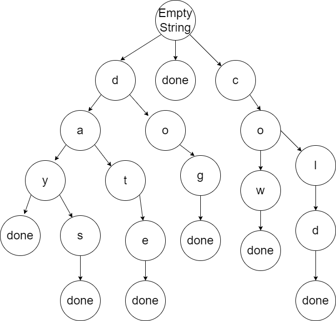
The diagram below shows an example of a Trie that stores words. Notice that the Trie begins with an empty character string and then branches out to all valid first letters for the values that are stored. Each branch represents a single letter. To find the words that are stored, you start at the root and progress downwards until you get to a letter that has done as a child. In many cases, additional words can be found by following other letters instead of stopping at the done. This Trie includes the words: “day”, “date”, “days”, “cow”, “cold”, and “dog”. Additionally, this Trie includes the empty string since done is connected to the root node.

When adding a new word, we start at the root and go one letter at a time. If the letter already exists in the Trie, then we goto the next letter. If the letter does not exist, then we create a child for that letter. The subsequent letters will all be new children.

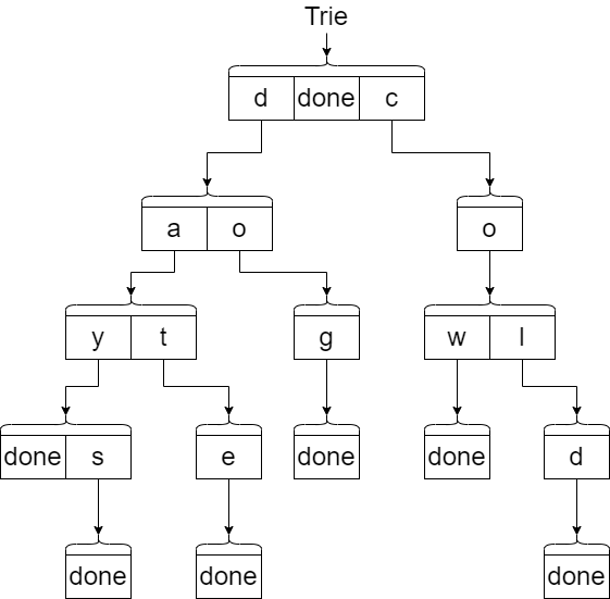
Unlike the binary search tree, the Trie can have a variable number of children. We can store those variable number of children in any data structure. For simplicity, we will use a dictionary as follows:

\(struct ~ ~ node\)

\(\quad \quad \lbrace string:Letter \looparrowleft node \rbrace ~ ~ or\)

\(\quad \quad \lbrace atom(done) \looparrowleft atom(nil) \rbrace.\)

\(\nonumber\)

The diagram below shows the same Trie example but with the perspective of dictionaries. Each set of boxes represents a separate dictionary. The arrows represent the \(node\) value associated with each key in the dictionary. Notice that we are not representing the empty string node but rather its implied.

Here is the specification for our add function:

\(spec ~ ~ add :: string ~ ~ node \rightarrow node.\)

\(\nonumber\)

When adding to the Trie, there are three scenarios that we must cover:

Add a word into an empty Trie (nil) - this will require that we create our root node represented as an empty dictionary (\(\lbrace \looparrowleft \rbrace\)). From this new root node, we will begin to add each letter of the word.
Check each letter (we will represent the word as a list of letters) to see if the letter already exists in the dictionary.
- If the letter does exist, then follow that node (the next dictionary) and check for the next letter recursively. We expect that as we follow the letter down that we will create new nodes so we will put the result of the recursion into the dictionary.
- If the letter does not exist, then create a new node (empty dictionary) for the letter and add it the current node dictionary. Follow that new node for the next letter recursively. Note that once we have this case, all subsequent letters will be new nodes as well.
If we run out of letters, then that means that the node we are on is a terminating node for a word. The value done should be added to the dictionary of this node (assuming it does not already exist). This is the base case.

All three scenarios appear in the definition below. Note that we are using three functions that we assume exists for a dictionary:

contains - Does the key exist in the dictionary
get - Get the value in the dictionary associated with the key
put - Put the key and value into the dictionary

\(de\mathit{f} ~ ~ add :: Word ~ ~ nil \rightarrow (add ~ ~ Word ~ ~ \lbrace \looparrowleft \rbrace);\)

\(de\mathit{f} ~ ~ add :: [] ~ ~ Node \rightarrow Node ~ ~ \text{when} ~ ~ (contains ~ ~ done ~ ~ Node) == true;\)

\(de\mathit{f} ~ ~ add :: [] ~ ~ Node \rightarrow (put ~ ~ done ~ ~ nil ~ ~ Node);\)

\(de\mathit{f} ~ ~ add :: [First|Rest] ~ ~ Node \rightarrow(put ~ ~ First ~ ~ (add ~ ~ Rest ~ ~ (get ~ ~First ~ ~ Node) ~ ~ Node) ~ ~\)

\(\quad \quad \text{when} ~ ~ (contains ~ ~ First ~ ~ Node) == true;\)

\(de\mathit{f} ~ ~ add :: [First|Rest] ~ ~ Node \rightarrow\)

\(\quad \quad (put ~ ~ First ~ ~ (add ~ ~ Rest ~ ~ \lbrace \looparrowleft \rbrace) ~ ~ Node).\)

\(\nonumber\)

The implementation of the add function will be left for an exercise.

In Erlang, we can use the following code to perform the contains, get and put operations on the dictionary. In Erlang, a dictionary is called a map Note that to create an empty map, we use #{}. If we wanted to prefill the map, we could use #{key1 => value1, key2 => value2, key3 => value3}.

Map = #{"Bob" => 10, "Sue" => 20},

% contains
true = maps:is_key("Bob", Map),
false = maps:is_key("Tim", Map),

% get
10 = maps:get("Bob", Map),
20 = maps:get("Sue", Map),

% put
New_Map = maps:put("Tim", 30, Map),
30 = maps:get("Tim", New_Map),

Problem Set 1

Starting Code: prove11_1/src/prove11_1.erl

Implement the add function and use the provided test code to verify the implementation. In the test code note that the pattern matching is done with := instead of => in Erlang. Also recall that Erlang will represent a string as a list of characters where each character is stored using the ASCII table integer value.

11.2 Searching and Counting

To search for a word in the Trie, we will check each letter to see if it is contained in the dictionary. Each check will be a recursive call. If the current letter is not in the dictionary, then the word does not exist. When we get through the whole word (base case with []) then we will need to look for done in the dictionary. If done does not exist, then the original word does not exist.

The specification and definition for the search function is given below:

\(spec ~ ~ search :: string ~ ~ node.\)

\(de\mathit{f} ~ ~ search :: Word ~ ~ nil \rightarrow false;\)

\(de\mathit{f} ~ ~ search :: [] ~ ~ Node \rightarrow (contains ~ ~ done ~ ~ Node);\)

\(de\mathit{f} ~ ~ search :: [First|Rest] ~ ~ Node \rightarrow (search ~ ~ Rest ~ ~ (get ~ ~ First ~ ~ Node)) ~ ~\)

\(\quad \quad \text{when} ~ ~ (contains ~ ~ First ~ ~ Node);\)

\(de\mathit{f} ~ ~ search :: [First|Rest] ~ ~ Node \rightarrow false.\)

\(\nonumber\)

The Erlang code for search function will be left for an exercise.

To count all the words in a Trie, we need to count all the nodes that have a done key in the dictionary. This will require recursion through all the keys in the dictionary. Prior to recusing through the keys in the dictionary, we will first need to determine if this node has a done key. If it does, then the total count will be 1 plus whatever is found in the recursive calls to each key in the node dictionary. Remember that the presence of a done key does not mean that there are no other key’s in the dictionary.

The specification and part of the definition is give below. The remaining definition and implementation will be left for an exercise.

\(spec ~ ~ count :: node \rightarrow integer.\)

\(de\mathit{f} ~ ~ count :: nil \rightarrow 0;\)

\(de\mathit{f} ~ ~ count :: Node \rightarrow\)

\(\quad \quad part\_of\_problem\_set\)

\(\quad \quad \text{when} ~ ~ (contains ~ ~ done ~ ~ Node) == true;\)

\(de\mathit{f} ~ ~ count :: Node \rightarrow\)

\(\quad \quad part\_of\_problem\_set.\)

\(\nonumber\)

Problem Set 2

Starting Code: prove11_2/src/prove11_2.erl

Implement the search function and use the provided test code to verify the implementation. You will need to copy the add function from the previous problem set.
Implement the remainder of the count function and use the provided test code to verify the implementation. Some additional information:
- In the starting code provided, you will note the following pattern matching syntax count(Node = #{done := nil}) -> which will match if the Node map provided contains a Key called done with a value of nil. This will still match even if there are other key value pairs stored in the map. Note that each time we match this pattern we should be adding 1 to the accumulated count.
- You may find the maps:fold function useful. In the same way that lists:foldl will call a lambda function to obtain an accumulated value from a list of values, the maps:fold will call a lambda function to obtain an accumulated value from a list of keys in the map. The lambda function for the maps:fold takes 3 parameters including the Key, Value, and previous Accumulator value. The maps:fold function can be used to iterate recursively through all the key value pairs in the Node map.

\(\nonumber\) \(\nonumber\)